
Equilibria & Oligopolies#
This section introduces the concept of equilibria in games, the paradigm of the prisoner’s dilemma, and oligopolies. These concepts are essential to understanding the models we will be studying the next sections, and for relating game theory to its economic applications.
Equilibrium#
The prisoner’s dilemma is a classic game first discussed by Merrill Flood and Melvin Dresher in 1950. In this game, there are two prisoners who have been captured and are being interrogated. The prisoners cannot contact each other in any way. They have two options: they can defect (betray the other prisoner to the police) or they can cooperate (maintain their silence). If both defect, both receive 4 years in prison. If one defects and the other does not, the defector goes free and the cooperator receives 5 years in prison. If both cooperate (meaning neither talks to the police), then they each receive 2 years in prison. We define mutual defection as the case when both prisoners defect and mutual cooperation as the case when both cooperate. The purpose of this game is to consider how a completely rational person would be best advised to proceed, and how different strategies for playing this game can be more or less effective.
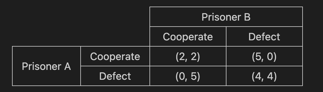
In the above payoff matrix, we see that if Prisoner A cooperates and Prisoner B defects, then Prisoner A gets 5 years in prisoner and Prisoner B gets none. It is important to note that the above payoff matrix is inverted; because we are talking about years in prison as opposed to utility, a higher value is worse for the player, and a player’s goal is to minimize their value in the payoff matrix, not maximize it as normally. We will use this payoff matrix convention when discussing the prisoner’s dilemma, but not with other games.
An important concept in game theory is finding the equilibrium of a game. There are different types of equilibria, but the most common one considered is the Nash equilibrium, named for the mathematician John Forbes Nash, Jr. (who you may remember as a character played by Russel Crowe in A Beautiful Mind). A Nash equilibrium occurs when no player can increase their own payoff by changing only their own strategy.
Definition
A Nash equilibrium is a set of strategy choices in a non-cooperative game in which each player, assumed to know the equilibrium strategies of the other players, has a chosen strategy and there can be no monotonic improvement; that is, no player can increase their payoffs by changing their strategy without another player changing their strategy.
Using this definition, what constitutes a Nash equilibrium for the prisoner’s dilemma? Well let’s consider the four possible combinations of strategies. (We use “D” as shorthand for “defect” and “C” for “cooperate” below.)
Prisoner A: C, Prisoner B: C. In this case, both Prisoner A and Prisoner B get 2 years. However, if Prisoner A’s strategy remains unchanged, Prisoner B can get fewer years in prison by changing to D, and vice versa. Thus, this is not a Nash equilibrium.
Prisoner A: D, Prisoner B: C. In this case, Prisoner B can change to D and lower their years from 5 to 4. Thus, this is not a Nash equilibrium.
Prisoner A: C, Prisoner B: D. As with (2), Prisoner A can change to D and lower their years in prison. Thus, this is not a Nash equilibrium.
Prisoner A: D, Prisoner B: D. In this case, if Prisoner A changes to C, then their years in prison increases from 4 to 5, as with Prisoner B. Neither player can increase their winnings (decrease their years in prison) by changing their strategy. Thus, this is a Nash equilibrium, with both Prisoner A and Prisoner B getting 4 years.
By describing the four states of the game, we see that only mutual defection is a Nash equilibrium of the prisoner’s dilemma.
Nash equilibria in payoff matrices
It is easy to use a payoff matrix to see which states, if any, are Nash equilibria. To see if a game state is a Nash equilibrium, the first value in the cell must be the maximum among all first values in that column and the second value must be the maximum across all second values in that row. This is because moving up and down a column represents changing the row-player’s strategy and moving along a row represents changing the column-player’s strategy. If these values are both maxima in their respective directions, then no player can obtain a better payoff by unilaterally changing their strategy, and we have a Nash equilibrium.
You can easily verify this by looking at the payoff matrix for the prisoner’s dilemma: the first 4 in mutual defection has the best payoff in the column and the second 4 has the best payoff in the row.
Oligopolies#
One of the most common applications of game theory in economics is the study of oligopolies, markets where the number of participants is limited. There are several examples of oligopolies that we experience without knowing in daily life: airlines, soft drinks, and telecom providers, to name a few. Oligopolies are different from regular markets in that they allow their participants to function similar to a monopoly by setting prices as a group; groups of participants conspiring on this kind of illicit activity are referred to as cartels.
Within oligopolies, however, we can observe competition more like a normal market as firms attempt to take market share from one another. When cartels set prices (by limiting the production of the good or service provided by their market), a firm can make a bid for market share by ignoring the agreed-upon production level and producing more. This has the effect of lowering the price of the good but the increase in production by the renegade firm will allow them to make up for the lost marginal revenue through increased sales volume. In this way, oligopoly members can compete against each other, making the market more and more competitive.
A prime example of this type of within-cartel competition was observed in the 2020 oil price war between Russia and Saudi Arabia. Both countries are members of OPEC (the Organization of Petroleum Exporting Countries), an oil cartel that consists of 12 member countries controlling 79% of the world’s oil reserves and 44% of oil production. OPEC sets oil prices by limiting the output of its member countries (a decrease in production results in higher prices).
The price war began when Saudi Arabia discounted its oil in response to Russia’s refusal to reduce production in accordance with OPEC’s directive. OPEC’s members had agreed to reduce oil production due to a low forecasted demand for oil due to the COVID-19 pandemic. When Russia (who was not an official member of OPEC but had agreed to cooperate with Saudi Arabia to manage oil prices) didn’t abide by OPEC’s decision, Saudi Arabia announced discounts on its oil, starting the price war and leading to a massive drop in the price of oil. We can see the effects of this price war by looking at the price per barrel of OPEC’s crude oil, plotted below.
The plot above marks the official start of the price war on March 8, 2020, in red. We see some precipitous drops both just before and for a while after the start of the price war, indicating the effect that it is having on oil prices. While there are some confounding variables here (hi there, COVID-19), we still see a serious drop in price that is not just attributable to the stock market volatility that experienced by the rest of the market in early 2020.