
IS-Curve#
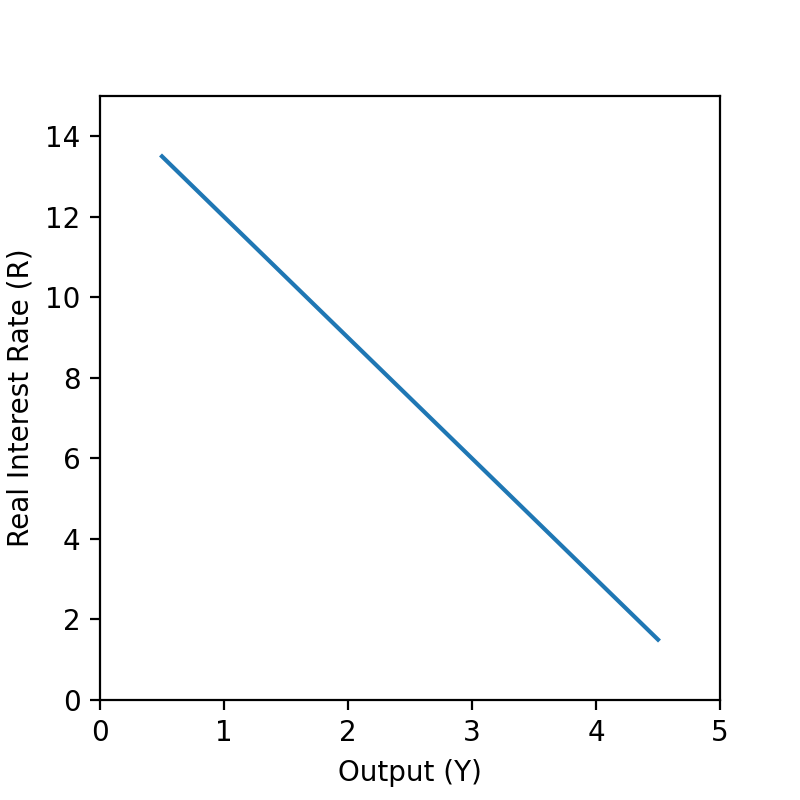
In this section we will introduce the IS curve (“investment–saving” curve), an important macroeconomics model that characterizes the relationship between real interest rates and output. The IS curve is downward sloping. When the real interest rate falls, output will increase. We will see why this inverse relationship is true and what this relationship implies for the economy.
[Figure - a downward slopign curve with Real Interest Rate on Y-Axis and Output on X-Axis]
Keynesian Cross#
First, we will discuss a model of aggregate demand and aggregate output. The Keynesian cross diagram, determines the equilibrium level of real GDP by the point where the total or aggregate demand in the economy is equal to the amount of output produced.
[Figure - Keynesian cross diagram with two upward sloping lines, Aggregate Demand on Y-xis and Output on X-axis]
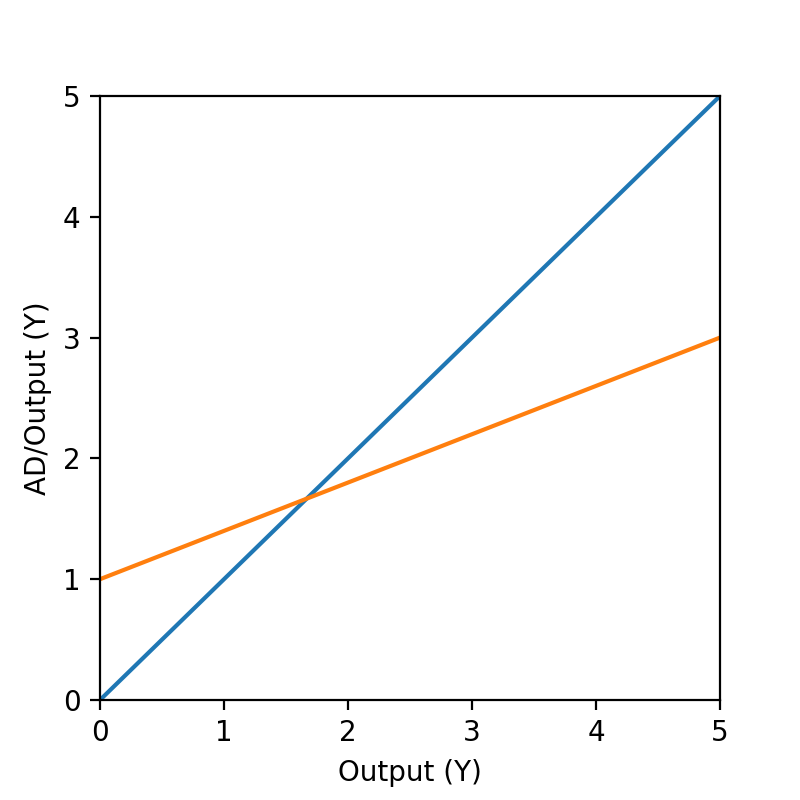
The axes of the Keynesian cross diagram show output / national income (or real GDP) on the horizontal axis and output / aggregate demand on the vertical axis. The orange line represents the aggregate demand, and the blue 45° line represents the aggregate output.
Why is the slope of the aggregate output line equal to 1?
Both the horizontal axis and the vertical axis are the output of the economy, so they should be the same.Why is the slope of the aggregate demand line less than 1, and the intercept greater than 0?
We will first consider how demand increases when national income rises. People can do two things with their income: consume it or save it (let’s ignore taxes for now). Each person who receives an additional dollar faces this choice. The marginal propensity to consume (MPC), is the share of the additional dollar of income a person decides to devote to consumption expenditures. Since the marginal propensity to consume is usually less than 1 (which means not all income is consumed), for every unit increase in national income, we will expect the aggregate demand to increase by less than 1 unit. So, the slope is less than 1.
However, even when the economy is not producing any output, people still need to consume. They may do so by using their savings or borrowing. So we have a positive intercept.
Dynamics of Keynesian Cross and Derivation of IS Curve#
Now, we are ready to derive the IS curve.
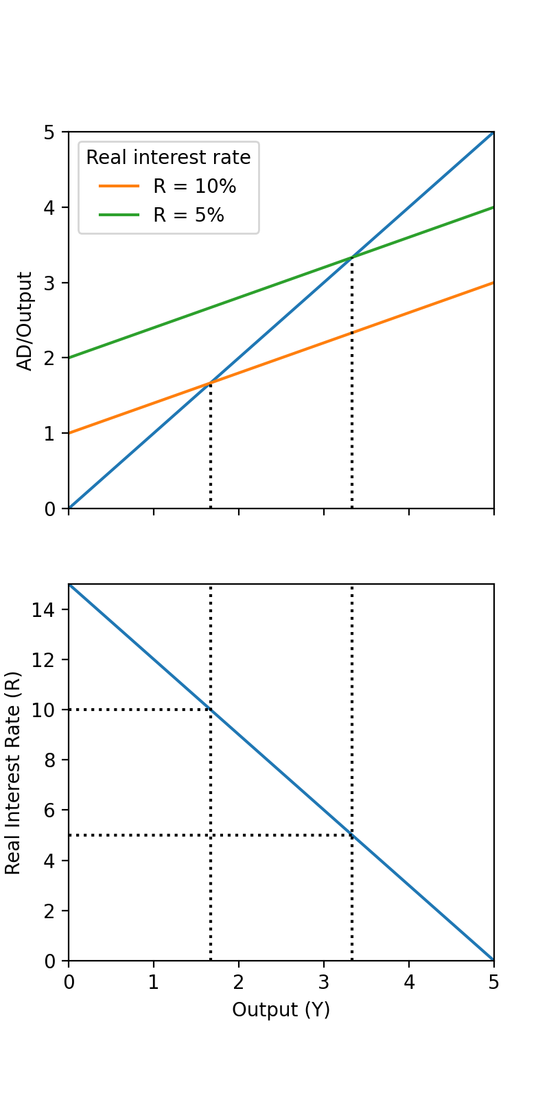
What will happen if the real interest rate decreases? First, people have less incentive to save money, since the gains from interest income are lower. Second, people have more incentive to spend (especially borrow money to spend) because the opportunity costs of spending are lower.
So, when the real interest rate decreases, people will tend to save less and consume more, shifting the aggregate demand curve in the Keynesian Cross upward. The equilibrium output level will therefore increase. The opposite direction will also hold true.
This precisely describes the inverse relationship between real interest rate and output.
[Figure - Kenesian cross diagram with interest rates at 10% or 5%]
Implication of IS Curve#
The IS curve explains the inverse relationship between real interest rate and output.
A more comprehensive model of how the money markets interact with the goods market can be illustrated by the IS–LM model. The IS–LM model, or Hicks–Hansen model, is a two-dimensional macroeconomic tool that shows the relationship between interest rates and the asset market (also known as real output in goods and services market plus money market). The intersection of the “investment–saving” (IS) and “liquidity preference–money supply” (LM) curves models a “general equilibrium” where equilibria simultaneously occur in both the goods and the asset markets. Hence, this tool is sometimes used not only to analyze economic fluctuations but also to suggest potential levels for appropriate stabilization policies.
The chart below illustates how each monetary and fiscal policy will affect the economy.
[Figure - four panel chart with different cases - IS downward sloping , LM upward sloping, interest reate on Y-axis, Income on X-axis, cases are A: Fiscal Expansion, B: Fiscal contration, C:Monetary Expansion, D: Monetary Contraction]
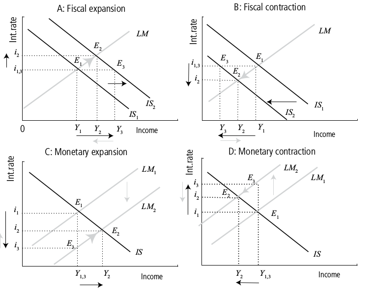
Source: Lev Lafayette, Chapter 2: The IS–LM model