
An Empirical Example from EEP 147#
Let’s take a look at an empirical example of production. The dataset for this section comes from EEP 147: Regulation of Energy and the Environment.
ESG_table = Table.read_table('ESGPorfolios_forcsv.csv').select(
    "Group", "Group_num", "UNIT NAME", "Capacity_MW", "Total_Var_Cost_USDperMWH"
).sort("Total_Var_Cost_USDperMWH", descending = False).relabel(4, "Average Variable Cost")
ESG_table
| Group | Group_num | UNIT NAME | Capacity_MW | Average Variable Cost |
|---|---|---|---|---|
| Old Timers | 7 | BIG CREEK | 1000 | 0 |
| Fossil Light | 8 | HELMS | 800 | 0.5 |
| Fossil Light | 8 | DIABLO CANYON 1 | 1000 | 11.5 |
| Bay Views | 4 | MOSS LANDING 6 | 750 | 32.56 |
| Bay Views | 4 | MOSS LANDING 7 | 750 | 32.56 |
| Old Timers | 7 | MOHAVE 1 | 750 | 34.5 |
| Old Timers | 7 | MOHAVE 2 | 750 | 34.5 |
| Big Coal | 1 | FOUR CORNERS | 1900 | 36.5 |
| Bay Views | 4 | MORRO BAY 3&4 | 665 | 36.61 |
| East Bay | 6 | PITTSBURGH 5&6 | 650 | 36.61 |
... (32 rows omitted)
This table shows some electricity generation plants in California and their costs. The Capacity is the output the firm is capable of producing. The Average Variable Cost shows the minimum variable cost per megawatt (MW) produced. At a price below AVC, the firm supplies nothing. At a price above the AVC, the firm can supply up to its capacity. Being a profit-maximising firm, it will try to supply its full capacity.
First, lets look at just the Big Coal producers and understand this firm’s particular behavior.
[Following image is a bar graph of 6 power plants ]
selection = 'Big Coal'
Group = ESG_table.where("Group", are.equal_to(selection))
Group
| Group | Group_num | UNIT NAME | Capacity_MW | Average Variable Cost |
|---|---|---|---|---|
| Big Coal | 1 | FOUR CORNERS | 1900 | 36.5 |
| Big Coal | 1 | HUNTINGTON BEACH 1&2 | 300 | 40.5 |
| Big Coal | 1 | REDONDO 5&6 | 350 | 41.94 |
| Big Coal | 1 | REDONDO 7&8 | 950 | 41.94 |
| Big Coal | 1 | HUNTINGTON BEACH 5 | 150 | 66.5 |
| Big Coal | 1 | ALAMITOS 7 | 250 | 73.72 |
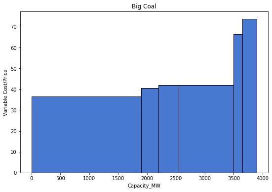
We have created the Big Coal supply curve. It shows the price of electricity, and the quantity supplied at those prices, which depends on variable cost. For example, at any variable cost equal to or above 36.5, the producer FOUR CORNERS (the one with the lowest production costs) will supply, and so on. Notably, we observe that the supply curve is also upward sloping since we need higher prices to entice producers with higher variasble costs to produce.
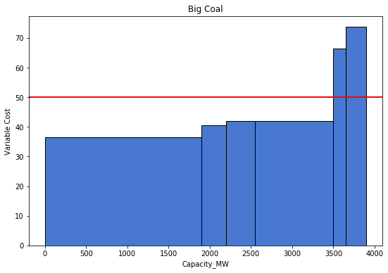
[Following image is a bar graph of 6 power plants with a price line]
Price: $30
No production

Price: $37
Total Production/Market Supply:  1900

Suppliers:  ['FOUR CORNERS']
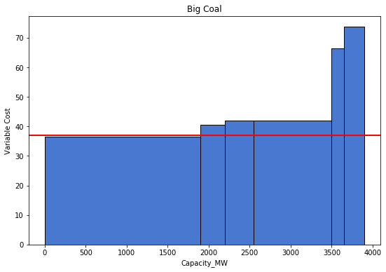
Price: $50
Total Production/Market Supply:  3500

Suppliers:  ['FOUR CORNERS' 'HUNTINGTON BEACH 1&2' 'REDONDO 5&6' 'REDONDO 7&8']
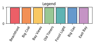
Now we will look at all the energy sources. They have been colored according to source for reference.
[Following image is a bar graph of all power plants in all portfilios ]
Price: $30
Total Production/Market Supply:  2800

Suppliers:  ['BIG CREEK' 'HELMS' 'DIABLO CANYON 1']

Price: $50
Total Production/Market Supply:  18650

Suppliers:  ['BIG CREEK' 'HELMS' 'DIABLO CANYON 1' 'MOSS LANDING 6' 'MOSS LANDING 7'
 'MOHAVE 1' 'MOHAVE 2' 'FOUR CORNERS' 'MORRO BAY 3&4' 'PITTSBURGH 5&6'
 'ORMOND BEACH 1' 'ORMOND BEACH 2' 'MORRO BAY 1&2' 'MANDALAY 1&2'
 'CONTRA COSTA 6&7' 'HUNTINGTON BEACH 1&2' 'PITTSBURGH 1-4'
 'EL SEGUNDO 3&4' 'ENCINA' 'REDONDO 5&6' 'REDONDO 7&8' 'COOLWATER'
 'ETIWANDA 1-4' 'SOUTH BAY' 'EL SEGUNDO 1&2' 'HUMBOLDT'
 'HUNTERS POINT 1&2' 'HIGHGROVE']
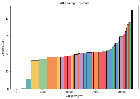
Look at the thin bars concentrated on the right end of the plot. These are plants with small capacities and high variable costs. Conversely, plants with larger capacities tend to have lower variable costs. Why might this be the case? Electricity production typically benefits from economies of scale: it is cheaper per unit when producing more units. Perhaps the high fixed cost required for electricity production, such as for equipment and land, is the reason behind this phenomenon.