
Taxes and Subsidies#
Now that we have discussed cases of market equilibrium with just demand and supply, also known as free market cases, we will examine what happens when the government intervenes. In all of these cases, the market is pushed from equilibrium to a state of disequilibrium. This causes the price to change and, as a result, the quantity transacted in the market.
Broadly, a tax is any type of financial charge imposed by the government, such as income tax, property tax, or excise tax. In this course, and for this section in particular, we will consider only taxes levied on consumption. These taxes are typically enforced on a state level in the US, and can take 2 forms:
An excise tax levies a fixed dollar amount on a particular good or service. A flat $1 tax per packet of cigarette sold is an example of an excise tax.
An ad valorem tax levies a percentage amount on the purchase of a particular good or service. For example the sales tax is an ad valorem tax.
Notably, consumption taxes can be levied on either the producer or the consumer. The side that pays for the tax upfront (when a transaction occurs) is known as the party that bears the statutory incidence of the tax. However, as you’ll soon learn, this does not mean that the party paying for the tax upfront bears the entire economic incidence of the tax.
A subsidy is the opposite of a tax; it involves either a monetary benefit given by the government or a reduction in taxes granted to individual businesses or whole industries.
Why Tax or Subsidize?#
The supply and demand models that we’ve examined so far do not necessarily reflect the entire picture; often, there are additional social costs or benefits associated with producing or consuming a good that is not paid for by a firm or considered by consumers.
For example, take a factory producing dyed color T-shirts that pollute a nearby river. In a world without government intervention, the firm would not have to clean up the river even though they should include factor that into their costs. This is an example of a negative externality, in which the private cost faced in production by a firm or consumption by a consumer is lower than the actual social cost.
[Following image is a hand drawn diagram of marginal social vs private costs]
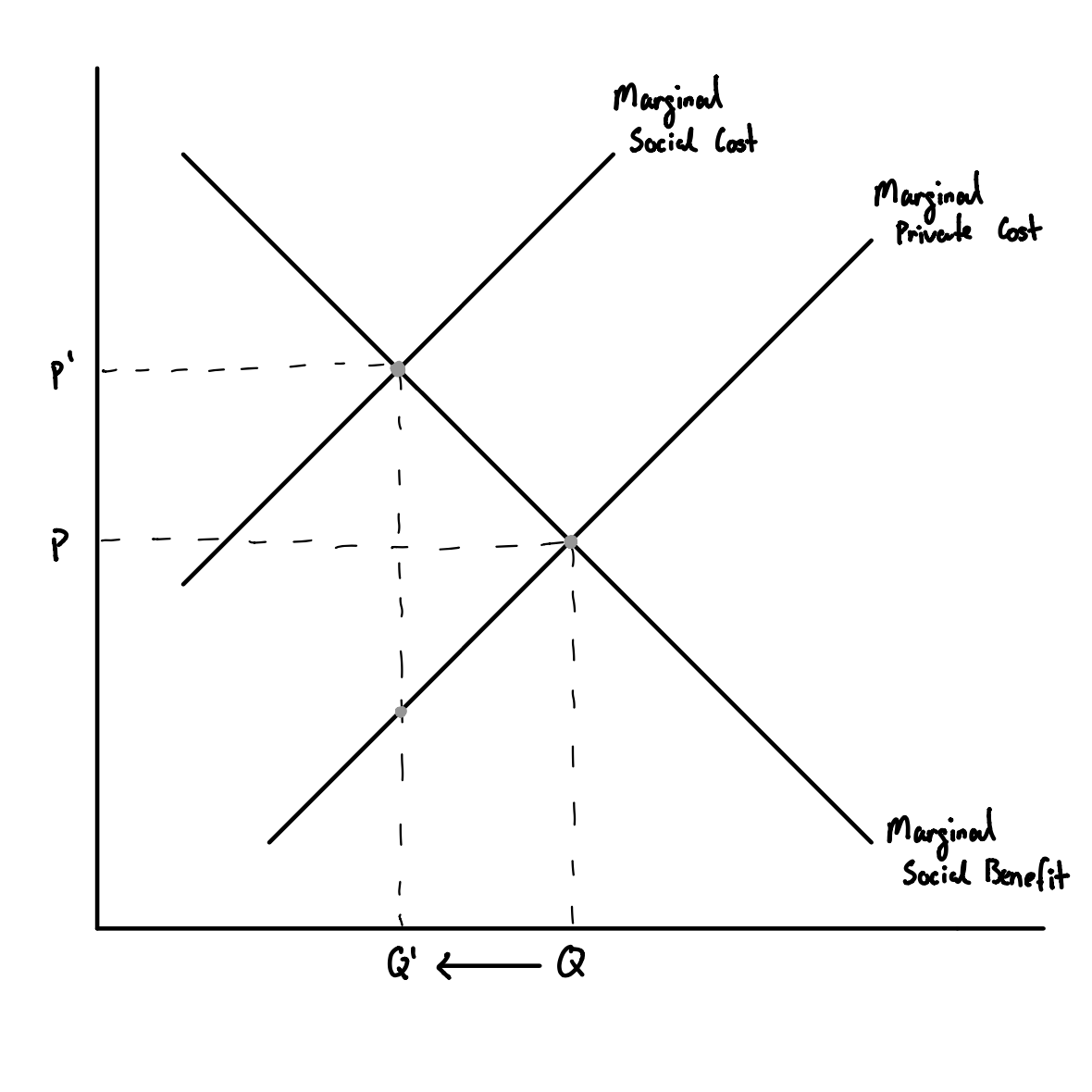
Fig. 4 A supply-side negative externality in which the marginal social cost is greater than the marginal private cost#
Take another example: vaccines. By consuming a vaccine shot, a consumer benefits their communities to overall reduce transmission of a disease. However, chances are the consumer probably did not consider the social benefits when making a decision on whether to vaccinate. This is an example of a positive externality, in which the private benefit faced in production by a firm or consumption by a consumer is lower than the actual social benefit (alternatively, in some cases it may be more intuitive to think about it as the private cost is greater than the social cost. Similarly, the opposite holds true for negative externalities).
[Following image is a hand drawn diagram of marginal social vs private benefit]
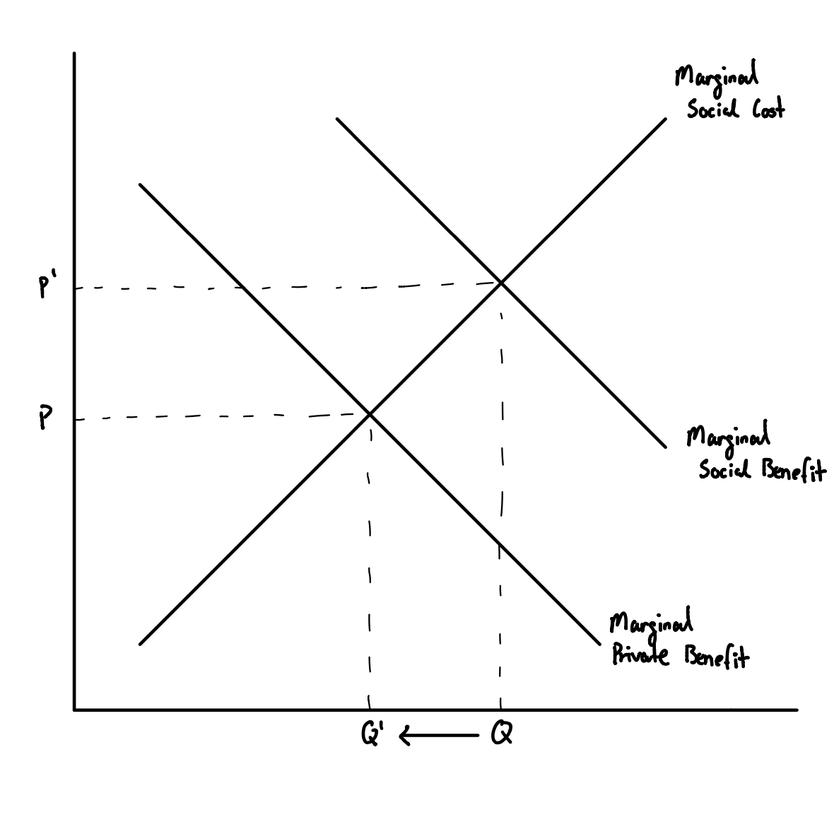
Fig. 5 A demand-side positive externality in which the marginal social benefit is greater than the marginal private benefit#
In this case, a market failure occurs, in which the true quantity demanded by society does not match what would occur in a free market without government intervention. This is where taxes and interventions come in: they can correct for externalities and thus resolve consequent market failures.
Effects of Taxation#
The primary method that governments use to intervene in markets to address negative externalities is taxation.
[Following image is a hand drawn diagram of supply shifting with a tax]
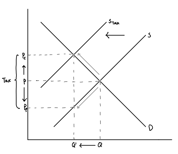
Fig. 6 A shift in supply due to a tax levied on producers#
If a tax is levied on producers, this decreases the quantity of goods they can supply at each price as the tax is effectively acting as an additional cost of production. This shifts the supply curve leftward. Compared to negative externality graph above, we can see that the tax essentially ‘corrects’ the supply curve based on the marginal private cost to instead mirror the supply curve based on the marginal social cost.
[Following image is a hand drawn diagram of demand shifting with a tax]
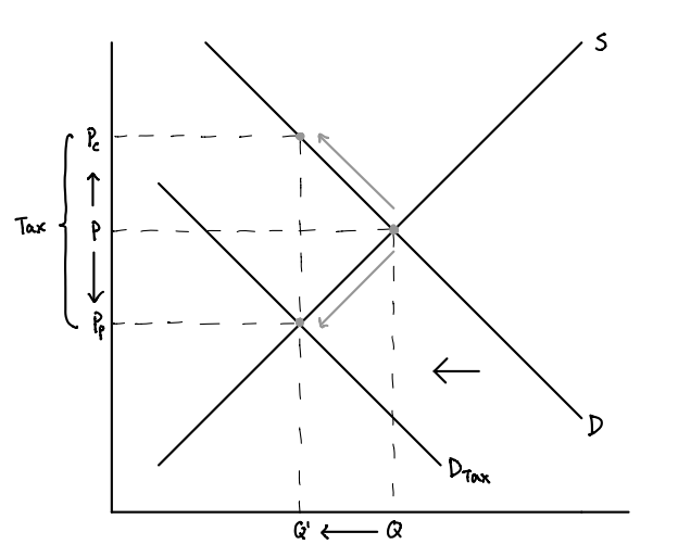
Fig. 7 A shift in demand due to a tax levied on consumers#
If the tax is levied on consumers, this increases the price per unit they must pay, thereby reducing quantity demanded at every price. This shifts the demand curve leftward.
Effects of Subsidies#
To account for positive externalities, a popular form of government intervention is a subsidy. They intend to lower production or consumption costs, and thus increase the quantity supplied of goods and services at equilibrium.
[Following image is a hand drawn diagram of supply shifting with a subsidy]
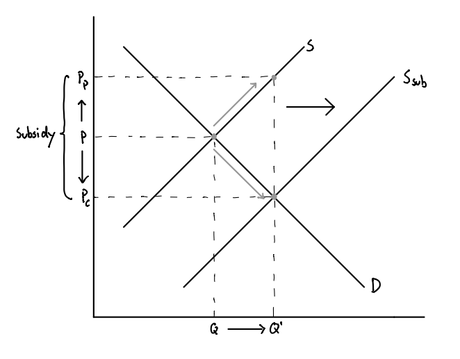
Fig. 8 A shift in supply due to a new subsidy#
We represent this visually as a rightward shift in the supply curve. As costs are lower, producers are now willing to supply more goods and services at every price. The demand curve remains unchanged as a subsidy goes directly to producers. The resulting equilibrium has a lower price
Consumer surplus increases as more individuals are able to purchase the good than before. Similarly, producer surplus has increased as the subsidy takes care of part (if not all) of their costs. Overall market surplus has increased.
The welfare gain is depicted in a similar way to that of a tax: a triangle with a vertex at the original market equilibrium and a base along
Examining the Effects of Taxes#
For the rest of this section, we will examine the effects of taxes in more detail.
[Following image is a hand drawn diagram of changes in surplus due to a change in Demand due to a tax]
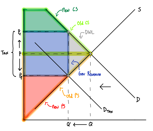
Fig. 9 Deadweight loss due to a tax levied on consumers#
The resulting equilibrium - both price and quantity - is the same in both cases. However, the prices paid by producers and consumers are different. Let us denote the equilibrium quantity to be
You will notice that the vertical distance between
Incidence#
Determining who bears the greater burden, or economic incidence, of the tax depends on the relative producer and consumer price elasticities. A good that consumers are relatively more inelastic towards (such that producers are more elastic) would mean that the burden of paying the tax will fall on consumers moreso than producers. Intuitively, this is because consumers are less sensitive to price changes and thus are ‘more willing’ to pay more to adjust to the tax. The opposite is true if the consumers are relatively more elastic (i.e. the producers are relatively more inelastic). See the figure below for more details.
One can calculate the burden share, or the proportion of the tax paid by consumers or producers:
Consumer’s burden share:
Producer’s burden share:
Graphically, the total tax burden is the rectangle formed by the tax wedge and the horizontal distance between 0 and
[Following image is a hand drawn diagram of supply shifts with different demand elasticities]
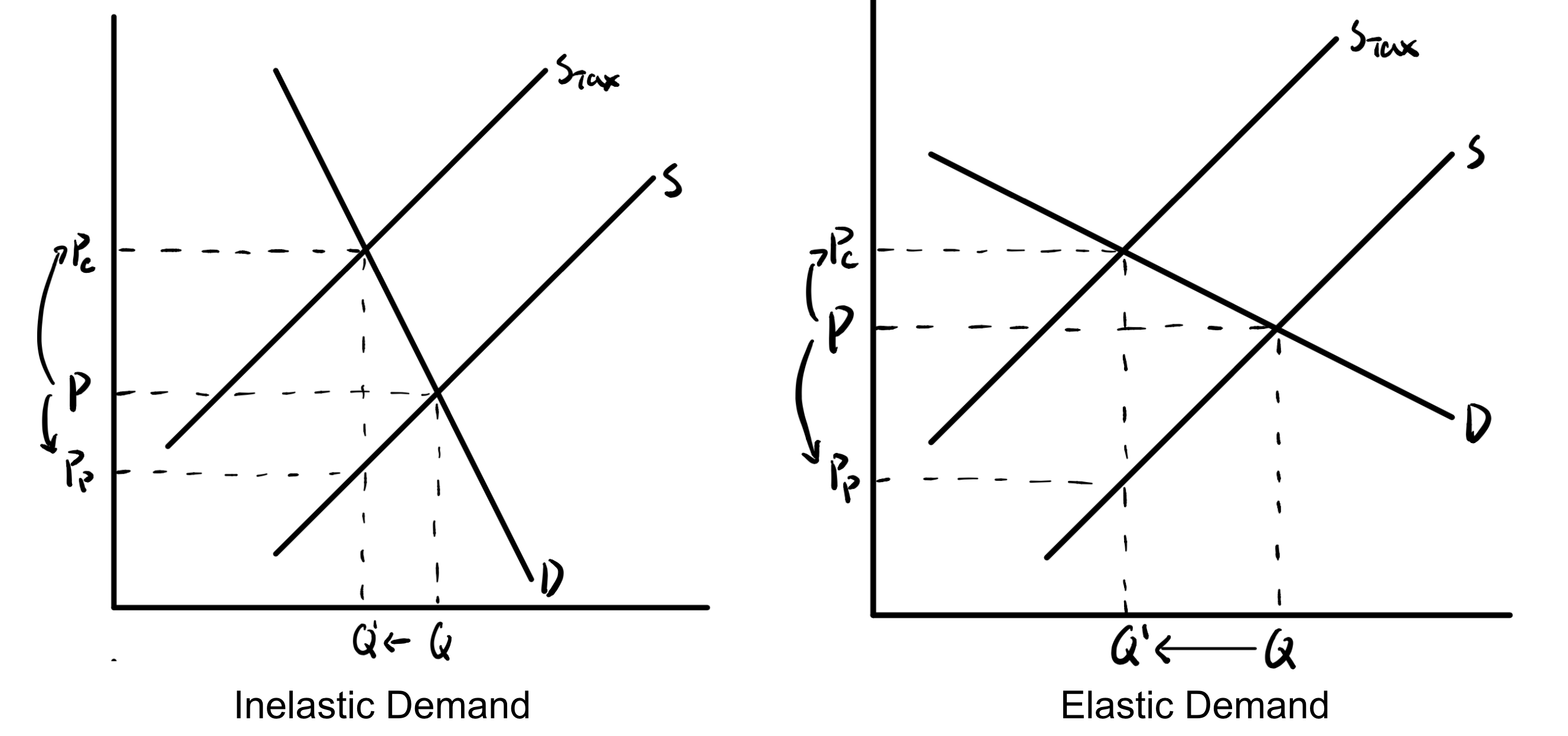
Fig. 10 Differences in economic incidences of a tax due to elastic and inelastic demand.#
Deadweight Loss#
Naturally, the introduction of the tax disrupts the economy and pushes it away from equilibrium. For consumers, the higher price they must pay essentially “prices” out some individuals - they are now unwilling to pay more for the good. This leads them to leave the market that they previously participated in. At the same time, for producers, the introduction of the tax increases production costs and cuts into their revenues. Some of the businesses that were willing to produce at moderately high costs now find themselves unable to make a profit with the introduction of the tax. They too leave the market. There are market actors who are no longer able to purchase or sell the good.
We call this loss of transactions: deadweight welfare loss. It is represented by the triangle with a vertex at the original market equilibrium and a base at the tax wedge. The area of the deadweight loss triangle, also known as Harberger’s triangle, is the size of the welfare loss - the total value of transactions lost as a result of the tax.
Another way to think about deadweight loss is the change (decrease) in total surplus. Consumer and producer surplus decrease significantly, but this is slightly offset by the revenue earned by the government from the tax.
We can calculate the size of Harberger’s triangle using the following formula:
Salience#
We noted in our discussion about taxes that the equilibrium quantity and price is the same regardless of whether the tax is levied on producers or consumers. This is the traditional theory’s assumption: that individuals, whether they be producers or consumers, are fully aware of the taxes they pay. They decide how much to produce or consume with this in mind.
We call the visibility at which taxes are displayed their salience. As an example, the final price of a food item in a restaurant is not inclusive of sales tax. Traditional economic theory would say that this difference between advertized or poster price and the actual price paid by a consumer has no bearing on the quantity they demand. That is to say taxes are fully salient. However, recent research has suggested that this is not the case.
A number of recent studies, including by Chetty, Looney and Kroft in 2009, found that posting prices that included sales tax actually reduces demand for those goods. Individuals are not fully informed or rational, implying that tax salience does matter.
Calculating Taxes Algebraically#
Expressing Quantity as a Function of Price#
So far, we have expressed our demand and supply curves using prices as a function of quantity, e.g.
To switch in between the different formats, we simply have to solve for the independent variable and express it in terms of our dependent variable. For
example, if demand is expressed as
Solving for the new quantity and price equilibria#
In previous weeks where there was no tax in the market, we could equate demand and supply to solve for the market price/quantity:
In reality, the demand function is based on the price consumers pay (which we’ll denote
In the no-tax scenario, the price received by producers is the same as the price paid by consumers. Hence, we are able to get away by expressing them both as
However, in the case of tax,
Because there are now 3 unknowns (
Once we are able to solve for
Lastly, to calculate the consumer burden, we seek to measure how much more the consumers are now paying due to the tax. Hence, this value is
An Example#
Part 1: Suppose the demand for rutabagas is
Solution
Since there is no tax,
Part 2: What is the equilibrium price with a per unit $2 sales tax?
Solution
With a $2 sales tax, we know that
Part 3: What are the tax burdens on the consumer and producer?
Solution
Consumer burden:
Producer burden:
This means that the consumer bears
Part 4: What is change in quantity transacted due to the tax?
Solution
Originally,
Now,
Note that we can also plug in