Introduction

The Financial Benefits of Your Major

Welcome to Data 88E: Economics Models! This class will explore the intersection of Data Science and Economics. Specifically, we will utilize methods and techniques in data science to examine both basic and upper-division Economics concepts. Throughout the course, we will consider a variety of economic problems both on the macro and micro level.

In the first demo of the course, we hope to give you a sense of the types problems you can expect to explore this semester by considering a problem that may be of personal relevance to you: the post-graduate incomes of different majors at Cal.

We will be using various visualization techniques to analyze the median incomes of different majors at UC Berkeley, in addition to the median incomes of those same majors at other colleges. If you forgot, the median income is the “middle” value: if you sorted all the individual incomes of a major in ascending order, the median would be the value that’s exactly in the middle. The median is also called the 50th percentile – at the median, exactly 50% of the individuals have an income lower than the median.

Do not be concerned if you don’t understand the code below: this entire exercise is purely a demo to motivate many profound concepts in Economics. If you’re interested, you may choose to come back to this demo at the end of the course and consider all the different techniques utilized in it - it’d be a great way of reflecting upon how much you’ve learnt!

Data Collection

Before we can use data science to tackle any issue, we must–well–obtain data (kind of mind-boggling, I know). Recall that we want to examine the median incomes of different majors at UC Berkeley as well as the median incomes of those same majors at other colleges. The term ‘other colleges’ is a fairly general one, and in this case we shall consider the average median incomes of those majors at alll other colleges in the United States.

In order to obtain a dataset, you can either collect it yourself (via surveys, questionnaires, etc.) or you can use datasets that others have gathered for you. In this demo, we are combining 3 different datasets:

• The median income for each major at Cal was obtained from Cal’s 2019 First Destination survey.

• The median income for each major overall was obtained from surveys conducted by the American Community Survey (ACS) from 2010 to 2012, a very popular data source for Economics Research! In the survey, ACS essentially calls college graduates and asked them their income as well as what they majored in at college. (As a side note, FiveThirtyEight later published this article:The Economic Guide to Picking a College Major using the results of the survey.) In this project, we will be using a modified version of the ACS survey - we will only be looking at the respondents who are 28 or younger. Can you think of why we would do this?

• The longitudinal data on long-run outcomes of UC Berkeley alumni was obtained from the University of California webpage. We will use this dataset later for a slightly different analysis.

Take a moment to consider the ways in which the 3 different datasets were created. Is it fair to draw direct comparisons between the datasets? What would be some potential issues and how could the differences in our datasets affect our analysis?

Mean vs Median

Before proceeding further, it is important to consider why we are choosing to look at the median, and not the average, income. In order to answer this question, let us think about what the distribution of incomes for a population would look like. Most likely, you would see a high amount of incomes around or slightly below the mean, with a few massive outlier incomes above the mean. For example, consider a theatre major who becomes a star on Broadway - while they’d be doing absolutely fantastic in their career, they are not representative of the average theatre graduate from Berkeley and would likely pull the average income way up. For this reason, using the median is more robust: it gives us a better idea of what the typical graduate for any major can generally expect to earn.

Now we’ll load in all the data. Take a look at the tables for each dataset. Note that P25th referes to the 25th percentile of incomes (the income level at which exactly 25% of incomes are lower) and P75th refers to the 75th percentile of incomes (the income level at which exactly 75% of incomes are lower). You may not know what all the different columns in the tables mean. That’s okay! As data scientists, we often encounter a lot of irrelevant data that we will discard later.

# Load in table of all majors' median incomes at Cal
cal_income = Table.read_table("cal_income.csv")
cal_income.show(10) 

Major	Cal Median	Cal P25th	Cal P75th
American Studies	55000	41600	60000
Anthropology	41600	36500	51000
Applied Mathematics	80004	65000	108000
Landscape Architecture	52000	45760	60000
Art	48880	38640	56390
Astrophysics	60000	50800	77182
Bioengineering	71000	54997	86500
Business Administration	75000	65000	85000
Chemical Biology	49920	44000	68000
Chemical Engineering	70000	65000	80000

... (39 rows omitted)

# Load in table of all other universities' average major median incomes
other_income = Table.read_table("recent-grads.csv") 
other_income.show(10)

Rank	Major_code	Major	Total	Men	Women	Major_category	ShareWomen	Sample_size	Employed	Full_time	Part_time	Full_time_year_round	Unemployed	Unemployment_rate	Median	P25th	P75th	College_jobs	Non_college_jobs	Low_wage_jobs
1	2419	PETROLEUM ENGINEERING	2339	2057	282	Engineering	0.120564	36	1976	1849	270	1207	37	0.0183805	110000	95000	125000	1534	364	193
2	2416	MINING AND MINERAL ENGINEERING	756	679	77	Engineering	0.101852	7	640	556	170	388	85	0.117241	75000	55000	90000	350	257	50
3	2415	METALLURGICAL ENGINEERING	856	725	131	Engineering	0.153037	3	648	558	133	340	16	0.0240964	73000	50000	105000	456	176	0
4	2417	NAVAL ARCHITECTURE AND MARINE ENGINEERING	1258	1123	135	Engineering	0.107313	16	758	1069	150	692	40	0.0501253	70000	43000	80000	529	102	0
5	2405	CHEMICAL ENGINEERING	32260	21239	11021	Engineering	0.341631	289	25694	23170	5180	16697	1672	0.0610977	65000	50000	75000	18314	4440	972
6	2418	NUCLEAR ENGINEERING	2573	2200	373	Engineering	0.144967	17	1857	2038	264	1449	400	0.177226	65000	50000	102000	1142	657	244
7	6202	ACTUARIAL SCIENCE	3777	2110	1667	Business	0.441356	51	2912	2924	296	2482	308	0.0956522	62000	53000	72000	1768	314	259
8	5001	ASTRONOMY AND ASTROPHYSICS	1792	832	960	Physical Sciences	0.535714	10	1526	1085	553	827	33	0.0211674	62000	31500	109000	972	500	220
9	2414	MECHANICAL ENGINEERING	91227	80320	10907	Engineering	0.119559	1029	76442	71298	13101	54639	4650	0.0573423	60000	48000	70000	52844	16384	3253
10	2408	ELECTRICAL ENGINEERING	81527	65511	16016	Engineering	0.19645	631	61928	55450	12695	41413	3895	0.0591738	60000	45000	72000	45829	10874	3170

... (163 rows omitted)

To make direct comparisons across majors, we combined all the tables above into a single one for us to use below.

majors = Table.read_table("cal_vs_all.csv")
majors.show(10)

Index	Major	Major Category	Median Income Difference	Cal P25th	Cal Median	Cal P75th	Overall P25th	Overall Median	Overall P75th
1	American Studies	Humanities & Liberal Arts	15000	41600	55000	60000	30000	40000	42000
2	Anthropology	Humanities & Liberal Arts	13600	36500	41600	51000	20000	28000	38000
3	Applied Mathematics	Computers & Mathematics	35004	65000	80004	108000	34000	45000	63000
4	Art	Arts	18380	38640	48880	56390	21000	30500	41000
5	Astrophysics	Physical Sciences	-2000	50800	60000	77182	31500	62000	109000
6	Bioengineering	Engineering	13900	54997	71000	86500	40000	57100	76000
7	Business Administration	Business	37000	65000	75000	85000	29000	38000	50000
8	Chemical Biology	Biology & Life Science	12520	44000	49920	68000	29000	37400	50000
9	Chemical Engineering	Engineering	5000	65000	70000	80000	50000	65000	75000
10	Chemistry	Physical Sciences	9000	37220	48000	61000	30000	39000	49900

... (39 rows omitted)

Our combined table above dropped the columns in above tables that we didn’t need to conduct our exploration. It has a column Median Income Difference: this column is the Berkeley median income minus the overall median income for each major. It gives us a sense of the value of Cal over the average university: the difference is the additional income we recieve from obtaining a Cal degree.

Before moving forward, take a second to consider how well the above tables would match with each other. For example, Electrical Engineering and Computer Science (EECS) is a popular major at Berkeley. However, the majors dataset didn’t have a direct equivalent for it. Instead, the majors dataset had Electrical Engineering, Electrical Engineering Technologies and Computer Engineering as separate majors. Since in theory students in EECS focus more on computer engineering, we chose to use the computer engineering data for drawing comparions in our final, combined table. However, there’s room for ambiguity here and that is another potential flaw in our exploration!

The below graph displays all the median salaries for all the majors in our dataset side by side. Feel free to look at the values for a few seconds - do you find anything interesting? [Following image is a bar chart of Median Incomes for Selected Majors]

The most lucrative major

Let’s imagine that Belfort is a freshman at Berkeley. Belfort is a very unique individual - he is someone who would be equally good at all majors and enjoys all majors equally. He also believes that money is the most important thing in the world. These assumptions are vastly oversimplifcations and not the case for anyone in real life; but in Economics you’ll find that we end up making significant simplifications to abstract away all the potential complications!

Since Belfort is equally good at and happy with all majors at Cal, the major he chooses is purely dependent on how much money he can earn after college with that major. Therefore, he will choose the major with the highest median income.

Let us sort our table by the Cal Median column in descending order to see which major that would be.

majors.sort('Cal Median',descending=True).show(10)

Index	Major	Major Category	Median Income Difference	Cal P25th	Cal Median	Cal P75th	Overall P25th	Overall Median	Overall P75th
15	Electrical Eng & Comp Sci	Engineering	55000	105000	115000	120000	45000	60000	75000
28	L&S Data Science	Computers & Mathematics	70200	90000	111500	120000	20000	41300	46000
27	L&S Computer Science	Computers & Mathematics	57000	103000	110000	120000	39000	53000	70000
30	L&S Ops Research & Mgmt Sci	Business	35250	75000	86250	106500	38000	51000	60000
39	Music	Arts	51000	51060	82000	121250	22300	31000	42000
3	Applied Mathematics	Computers & Mathematics	35004	65000	80004	108000	34000	45000	63000
48	Statistics	Computers & Mathematics	35000	61000	80000	107000	26700	45000	60000
35	Materials Science & Eng	Engineering	28000	72700	80000	84000	35000	52000	62000
24	Industrial Eng & Ops Rsch	Engineering	23000	72250	80000	87500	37900	57000	67000
16	Engineering Physics	Engineering	22000	65250	80000	100000	25000	58000	74000

... (39 rows omitted)

However, what if instead of just wanting the maximum amount of cash after college, Belfort was super proud of getting into Berkeley and instead wanted to maximise the amount of additional benefit he recieves from attending Berkeley over other universities? Let’s sort our table by the Median Income Difference column in descending order to see which major would give Belfort the highest additional income from going to Berkeley.

Do any values in either of our sorted table surprise you? Why might that be?

majors.sort("Median Income Difference",descending=True).show(10)

Index	Major	Major Category	Median Income Difference	Cal P25th	Cal Median	Cal P75th	Overall P25th	Overall Median	Overall P75th
28	L&S Data Science	Computers & Mathematics	70200	90000	111500	120000	20000	41300	46000
27	L&S Computer Science	Computers & Mathematics	57000	103000	110000	120000	39000	53000	70000
15	Electrical Eng & Comp Sci	Engineering	55000	105000	115000	120000	45000	60000	75000
39	Music	Arts	51000	51060	82000	121250	22300	31000	42000
7	Business Administration	Business	37000	65000	75000	85000	29000	38000	50000
30	L&S Ops Research & Mgmt Sci	Business	35250	75000	86250	106500	38000	51000	60000
3	Applied Mathematics	Computers & Mathematics	35004	65000	80004	108000	34000	45000	63000
48	Statistics	Computers & Mathematics	35000	61000	80000	107000	26700	45000	60000
12	Cognitive Science	Biology & Life Science	34000	53000	75000	105000	20000	41000	60000
43	Physics	Physical Sciences	29364	54996	74364	100000	30000	45000	68000

... (39 rows omitted)

Let’s now do the opposite and sort our table by the Median Income Difference column in ascending order.

majors.sort("Median Income Difference").show(10)

Index	Major	Major Category	Median Income Difference	Cal P25th	Cal Median	Cal P75th	Overall P25th	Overall Median	Overall P75th
40	Nuclear Engineering	Engineering	-2150	57625	62850	80675	50000	65000	102000
5	Astrophysics	Physical Sciences	-2000	50800	60000	77182	31500	62000	109000
9	Chemical Engineering	Engineering	5000	65000	70000	80000	50000	65000	75000
41	Nutritional Science	Health	6200	36500	41200	49980	26000	35000	45000
13	Conserv & Resource Stds	Agriculture & Natural Resources	6600	37580	41600	57020	25000	35000	42000
10	Chemistry	Physical Sciences	9000	37220	48000	61000	30000	39000	49900
22	Geography	Social Science	10000	35000	48000	60000	30000	38000	50000
32	L&S Social Welfare	Psychology & Social Work	10000	35520	40000	50000	25000	30000	35000
25	Integrative Biology	Biology & Life Science	10280	33280	43680	56160	24000	33400	45000
21	Forestry and Natural Resources	Agriculture & Natural Resources	10600	35360	45600	51000	28600	35000	48000

... (39 rows omitted)

As you can see in the table, the median income difference for both nuclear engineering and astrophysics is negative. This is rather peculiar, especially since Cal has great programs for both those majors. Why would Cal graduates earn less income than the graduates of the average college for those 2 majors?

Hint: consider what each of our datasets describes. Is it an apples-to-apples comparison?

The answer is because the dataset with the median incomes for all colleges actually described recent graduates (people who are 28 and younger, rather than just fresh college graduates. It is likely that most people who graduate with Nuclear Engineering and Astrophysics degrees in other colleges tend to stay in the industry for their fields and keep accumulating experience. This would explain why a dataset that includes data from 28 year olds would have a higher median income than fresh Cal graduates in the same field.

Generalization and Causal Inference

While Belfort would be equally good at and enjoy all majors equally, the implications for him may not generalize for anyone else.

If you decide to major in EECS, it does not mean that you will have more income post-grad than that from majoring in anything else. For example, someone who is a fantastic artist but not very good at computer science would probably make far more money majoring in art than in EECS. In addition, just because EECS has the highest median income overall doesn’t mean that any individual is guaranteed a high median income if they decide to major in EECS. Overall, our results are not completely generalizable to others.

The causal effect of majoring in EECS on incomes may also be overstated. Consider the fact that those who major in EECS tend to come from families whose parents are already in working in tech. As a result, these students will likely also find better jobs post-grad. This is what we call a confounding variable – it is positively correlated with our treatment variable of majoring in EECS. If we do not observe this confounding factor, our analysis would likely overstate the effect of an EECS degree on post-grad incomes.

A brief discourse on utility

From seeing our results, you may be wondering: why doesn’t everyone just major in EECS then?

For Belfort, money is the only thing in the world that derives happiness. However, this is once again an oversimplication for the vast majority of people in the real world. People derive utility from sources other than just their bank account; often, we choose relatively lower-paying jobs in order to derive more happiness in our lives.

Utility is a measure of ‘satisfaction’ or ‘happiness’ when we consume a good, while disutility is a measure of ‘unsatisfaction’ or ‘harm’ when we consume a bad. In economics, one assumption we will always make is that people will always seek to maximize their utility and minimize their disutility.

However, we encounter diminishing marginal utility as we consume more and more of a good. For example, the utility of the first cookie you eat is likely much higher than the 20th cookie you eat. Similarly, we may encounter increasing marginal disutility as we consume more and more of a bad. For example, the disutility of the first hour doing something you dread is probably not as bad as the 10th hour of doing something you dread.

For many of us, money provides a source of utility, while working or the studying required to get there may provide a source of disutility. This presents a tradeoff: for some, the disutility from studying EECS or working as a programmer greatly outweights the utility from the money. Perhaps another job in a different field requires significantly lower disutility to achieve, without much impact on the utility of the income associated with it. This phenomenon would explain why not everyone decides to major in EECS!

Incomes Over Time: Computer Science vs Economics

So far our exploration of the data has considered a rather general timeframe of “post graduation”, but perhaps it would be more insightful if we dove in and took a look at how incomes differed across various ages. We can do so using the table below that consists of data collected by the UC ClioMetric History Project. By compiling a database of digital student transcripts of all UC undergraduates and then linking California wages to individuals in the transcript database, they were able to produce comprehensive dashboards that visualize demographics, major choices, and long-run incomes of each UC campus’s alumni over the past 70 years.

You can learn more about how they collected the data in Incomes Over Time , but for now we will just focus on a snapshot of the data. In particular, we are interested in exploring how percentile incomes compare between Cal alumni who majored in computer science versus those who majored in economics. Run the following cell to check it out.

cs_vs_econ=Table.read_table("cs_econ_by_age.csv")
cs_vs_econ.show(10)

Age	CS 90th Percentile	CS 75th Percentile	CS Median	CS 25th Percentile	Econ 90th Percentile	Econ 75th Percentile	Econ Median	Econ 25th Percentile
23	176659	137090	106548	79617	117187	90009	69737	52210
24	222420	157764	118886	92054	127454	100859	81425	62719
25	232527	165109	128178	103616	151641	114465	90069	69207
26	261114	175940	132967	105601	166973	125092	97294	74010
27	261653	172378	132357	104193	176418	131773	102361	75553
28	252461	175559	135852	107205	192756	140982	107022	76929
29	259180	180283	141214	111220	207451	153648	115540	82523
30	276090	193007	148817	118115	235170	168052	123457	87689
31	299140	203522	154232	121146	254526	177747	129407	90303
32	314279	212274	160000	126626	279246	187899	135302	93089

... (30 rows omitted)

Here we have a table where each row corresponds to a certain age. It begins with age 23 (typically how old people are when getting their first job out of college), and goes up until age 62 (when people retire from the workforce).

Let’s graph our data using some line plots: line plots are especially useful when trying to visualize trends that change over time.

Run the following cell to visualize the data. The yellow lines correspond to CS incomes, while the blue lines correspond to Econ incomes.

[Following image is a graph of “Comparing Incomes of Computer Science Majors vs Economics Majors”]

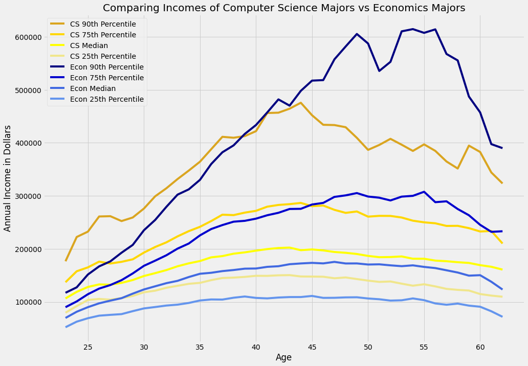
Let’s take a look at how the incomes compare at each percentile. The most notable trend is probably the fact that for the most the part, CS majors typically make more money than Econ majors. We especially observe this trend in the 25th and 50th percentiles, and this follows accordingly with our exploration earlier in the notebook that students who majored in L&S Computer Science on average had a higher median income than pretty much every other major.

The graph above helps explain why CS is one of the most popular majors here at Berkeley. Software engineering and related disciplines have a huge demand for fresh talent, so that individuals entering these fields are duly compensated. This in and of itself is a big appeal of students wanting to major in computer science.

Right off the bat out of college, fresh CS graduates are looking at a six figure income: even the 25th percentile of CS majors are making over $103,000 by the time they are 25. At any given percentile level, CS graduates outearn their Economics counterparts immediately post-graduation.

Intertemporal Effects

However, we don’t just choose our majors based off of the immediate post-graduation income. Intuitively, we would want to maximize our total lifetime income we make. This idea is called intertermporal utility maximization: Economists often take into account one’s utility across all possible time periods.

Considering lifetime income, which major would be better? Well, it depends: if you are at the bottom 25th or 50th percentile, CS is better. This suggests that the typical Economics major will likely never outearn the the typical CS major.

However, we observe that Economics majors at higher percentiles ultimately overtake CS majors in earnings. Intuitively, this should make sense. Perhaps top Economics majors are more likely to become successful executives later on in their careers while make more money than top CS majors, who continue to stay as software engineers or become engineering managers.

Risk

We observe that Economics majors have a much larger spread in their lifetime earnings than CS majors: top Economics graduates make significantly more than bottom Economics graduates, compared to top CS and bottom CS graduates.

This brings to the light the notion of risk. Majoring in CS carries relatively lower variance: whether you are a top notch developer in the 75th percentile or a subpar developer in the 25th percentile, you will probably make a solid living. Since most CS majors typically end up pursuing similar careers in the realms of software development, there is less variance in the occupations. There is also less risk: most CS majors can expect to land a software engineering job and continue working as one twenty years into their career.

The same story is less true for Economics majors: a top-notch Economics major will significantly out-earn a subpar Economics major. This is partly due to the vastly differing occupation types Economics majors become: analysts, bankers, consultants, just to name a few (Economics is a very versatile degree, afterall). Twenty years down the line, the top Economics majors will have higher ceilings perhaps with a lot of opportunity for leadership or executive positions. There is a lot more variance in the types of jobs and thus salaries that Economics majors will attain. In addition, there is a lot more risk: not every Economics major will become a top executive, and most end up with more ‘average’ jobs that earn less than that of similar percentile CS majors.

This means that if you know you are at the top regardless of your major, you will tend to ultimately earn more income as an Economics major than a CS major. But a caveat: it’s impossible to guarantee that you will be in the top, no matter how hard you work. Often, life has uncertainties and involves a great deal of luck to become successful.

The table and graph above only considered the percentile incomes of CS and Economics majors, but if you’re interested in drawing more comparisons, check out Long Rund outcomes for UC Berkeley Alumni. You can compare between all types of popular majors at UC Berkeley, and even toggle around with more features like gender, ethnicity, or even specific courses.

An Afterword

In this demo, we’ve covered a series of fundamental Economics ideas such as income, utility, and risk. We’ve also gone over a series of more statistical concepts that are also at the heart of empirical Economics such as causal inference, generalization, and unobserved variables. We did this all using data science techniques and visualizations, while being cognizant of potential sources of error. We will be revisiting a lot of these themes in later parts of the course.

From this exercise you may have noticed that pursuing either Economics, Data Science, or both are great options in terms of post-graduation incomes. This means you’ve probably chosen wisely to have ended up in this class.

Welcome to Data 88E!