Demand Curves

In this chapter, we will explore one of the most foundational yet important concepts in economics: demand curves. The demand curve shows the graphical relationship between the price of a good or service and the quantity demanded for it over a given period of time. In other words, it shows the quantity of goods or services consumers are willing to buy at each market price. The quantity of goods or services demanded or supplied can be modeled as a function of price, as in:

\[\text{Quantity} = f(\text{Price})\]

Notably, the curve is downwards sloping because of the law of demand, which states that as the price of a good or service increases, the quantity demanded for it decreases, assuming all other factors are held constant.

This should make intuitive sense: as prices increase, fewer people are willing to pay the higher price for the same good. On the other hand, as prices decrease, more people are willing to pay the lower price for the same good. Hence, the quantity demanded of a good or service has an inverse relationship with the price.

For now, let’s assume that the relationship is somewhat linear and can be described as

\[\text{Quantity}_{d}=-a \cdot \text{Price}_{d} + b\]

We can interpret the equation above as follows: as the price of a unit increases by 1, there is an \(a\) unit decrease in the quantity demanded. For example, \(\text{Quantity}_{d}=-2 \cdot \text{Price}_{d} + 3\) would suggest that a price increase by 1 would decrease overall quantity demanded in the market by 2.

Price can also be measured as function of quantity to denote demand. In this case, we use an inverse demand function, as it is the inverse function of the demand function above. Since price is a function of quantity,

\[\text{Price} = f(\text{Quantity})\]

As we are solving for the inverse of the previous demand function, the inverse demand function for the example above is

\[\text{Price}_{d}=-\frac{1}{2} \cdot \text{Quantity}_{d} - \dfrac{3}{2}\]

Movement and the Demand Curve

Shifts in the Demand Curve

The demand curve can shift in or out based on exogenous events that occur outside of the market. Some factors other than a change in price of the good/service could be changes in:

• buyer’s income

• consumer preferences

• expectation of future price/supply/demand

• changes in the price of related goods

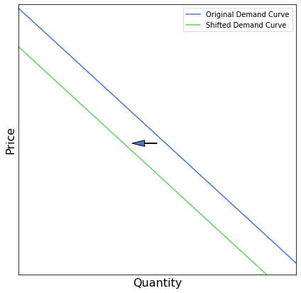
If any of these changes occur and causes the demand for the selected good/service to decrease, then the curve shifts to the left as less of the good or service will be demanded at every price. Similarly, if any of these changes causes the demand for the selected good/service to increase, the curve would shift to the right. This signifies that more of the good or service will be demanded at every price. For example, consumers’ incomes decreased during the 2008 recession, thus decreasing overall buying power and shifting the demand curve leftwards; a left shift in the demand curve suggests that consumers would purchase fewer quantities of goods at every price.

[Following image is a graph of a shifting demand curve]

Movements along the Demand Curve

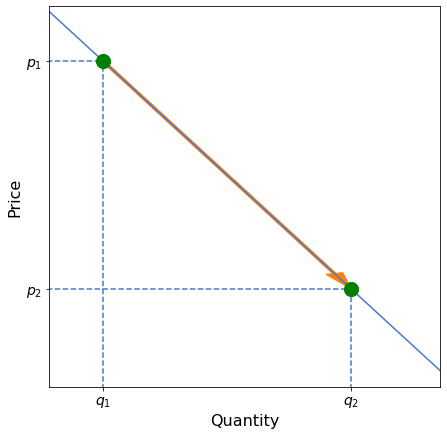
Above, we looked at when exogenous events affect the demand curve. Another concept is movements along the demand curve, which would be considered endogenous events. In movements along the demand curve, changes in price affect the quantity demanded of the good or service. This assumes ceteris paribus, which means holding all other factors constant. This phenomenom is called the Movement of the Demand Curve. With a change in price, the quantity demanded for the good or service can shift the quantity demanded either upward or downward on the demand curve. For example, consider the shift on the graph below from quantity \(q_1\) at price \(p_1\) to quantity \(q_2\) at price \(p_2\).

[Following image is a graph of a shift along a demand curve]

Income and Substitution Effect

Changes in the price of a good also leads to 2 effects, which can help explain the law of demand:

• Income Effect: Examines how the change in price of the good affects income, which then affects the quantity demanded of a good or service. If the price of a good increases, it would require the consumer to spend more of their income on the good. This dissuades consumers from purchasing more of the good, decreasing the quantity demanded. If the price of a good decreases, consumers would spend less money to receive the same good. This increases the quantity demanded for the good, because consumers would have more income remaining to purchase additional units, given the increase in the amount of purchasing power required to obtain the good.

• Substitution Effect: Examines how the change in price of the good affects its demand relative to other goods and services. If the price of a good increases, then consumers might look at similar goods that function in the same way or yield an equivalent amount of utility as the original good. Consumers are effectively shifting or substituting away from the relatively more expensive good to a cheaper alternative, thereby decreasing the quantity demanded for the original good. The converse is also true: if the price of a good decreases, then consumers that currently purchase other similar goods might start consuming this good instead, because it would cost less money for them to obtain.

For example, if the price of gas increases, the higher price for gas might encourage consumers to look at purchasing more efficient cars, such as electric or hybrid cars, thus decreasing the demand for gas. This is the subsitution effect. If the consumer stays with their original car, then they would have less disposable income after purchasing the now-more-expensive gas, so they might purchase less gas. This is the income effect.